


Next: Help
Up: xi3: Tuning Program for
Previous: xi3: Tuning Program for
Here is a sample procedure showing how to use xi3 in practice.
We are looking at the problem of 8 particles at SC lattice sites
in (5, 5, 5) periodic box.
A sample configuration file (xi3.scm) is given in the package:
; sample set file for xi3
; SC lattice config of 8 particles in (5,5,5) box
; $Id: manual.tex,v 1.5 2008/10/12 20:16:53 kichiki Exp $
(define version    "F")     ; version. "F", "FT", or "FTS"
(define flag-mat   #t)      ; #t => matrix scheme, #f => atimes scheme
(define flag-notbl #f)      ; #t => no-table,      #f => with table

(define np         8)       ; number of particles
(define ewald-eps  1.0e-12) ; cut-off limit for Ewald summation

; lattice vector
(define lattice '(5.0  5.0  5.0))

; configuration of particles
(define x #(
0.0  0.0  0.0
2.5  0.0  0.0
0.0  2.5  0.0
0.0  0.0  2.5
0.0  2.5  2.5
2.5  0.0  2.5
2.5  2.5  0.0
2.5  2.5  2.5
))

; list of time ratio Tr/Tk for Ewald summation (optional)
;(define ewald-trs
;  '(0.1
;    1.0
;    10.0
;    100.0
;    ))
Here is a part of the result:
# F version table matrix
0.110000 0.245379 22.087 21.575 0.512 1.33163581314065055e-01 2197 125 1713 80
0.121000 0.249308 21.106 20.592 0.514 1.33163581314059309e-01 2197 125 1713 80
0.133100 0.253300 20.812 20.224 0.588 1.33163581314069690e-01 2197 125 1689 92
...
Each line of the output consists of 10 columns in this case,
that is, for F version with table.
First 5 columns are the same for any cases;
First and second columns are  and
and  (see below in details).
The next 3 are CPU times in milli-seconds
for real space, reciprocal space, and the total
calculations, respectively.
The next column is, for F version, the averaged velocity
obtained by the calculation (see below in details).
For FT and FTS versions, there are 2 and 3 numbers there.
Next two integers show the lattice points within the range
for real and reciprocal summations. Note that the numbers
are those in the cubic regions (not spherical). For non-table version
we are taking into account the lattice points within the cubic region
specified by the numbers of lattice points in
(see below in details).
The next 3 are CPU times in milli-seconds
for real space, reciprocal space, and the total
calculations, respectively.
The next column is, for F version, the averaged velocity
obtained by the calculation (see below in details).
For FT and FTS versions, there are 2 and 3 numbers there.
Next two integers show the lattice points within the range
for real and reciprocal summations. Note that the numbers
are those in the cubic regions (not spherical). For non-table version
we are taking into account the lattice points within the cubic region
specified by the numbers of lattice points in  ,
,  , and
, and  directions.
For table version, on the other hand, we apply more complicated
(and empirical) criteria for the truncation of lattice sum and
roughly speaking this reduce the region from cubic to spherical.
In the case, the final two integers, which are the actual numbers
of points for real and reciprocal summations we took, are added.
directions.
For table version, on the other hand, we apply more complicated
(and empirical) criteria for the truncation of lattice sum and
roughly speaking this reduce the region from cubic to spherical.
In the case, the final two integers, which are the actual numbers
of points for real and reciprocal summations we took, are added.
In xi3 program as well as libstokes
library, another parameter instead of is used.
is a rough estimation of CPU time ratio between real and reciprocal
summations and related to as
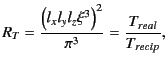 |
(2.31) |
where
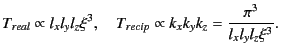 |
(2.32) |
Figure 2.1:
versus .
|
|
Figure 2.1 shows vs. .
(Those are at the first and second columns in the result file.)
Note that this is implemented in the routine
xi_by_tratio ().
Changing , the number of lattice points in real and reciprocal
summations are changing: The former is decreasing
and the latter increasing as is increasing.
Because the calculation result is independent of and therefore ,
we can use this parameter to tune the calculation of the Ewald summation.
That is, we can take a specific value of which minimize
the calculation cost.
This is the whole purpose of xi3 program.
Figure 2.2 shows CPU times for real and reciprocal spaces
and the total.
As we see, there is an obvious minimum point on the total CPU time.
In this example (for SC lattice of  particles in
 periodic box),
the minimum is around
periodic box),
the minimum is around
 .
.
Previously, I wrote that
the calculation result is independent of and therefore .
This is the mathematical conclusion and therefore this is a good
check for the code:
The results should be the same for various (and therefore ).
Actually, we truncate the lattice summations at the point where
the term is small enough. The criteria is given by another parameter
ewald_eps.
In this example, we take
 .
(Small enough, isn't it?)
In the code of xi3, we calculate not physical problems
but the plain
.
(Small enough, isn't it?)
In the code of xi3, we calculate not physical problems
but the plain
 calculation
for the mobility matrix
calculation
for the mobility matrix
 and
a vector
and
a vector
 .
The 6th column of the result xi3 generates
is the average of
, that is,
a kind of averaged velocity. (``a kind of'' means
that the average is taken element-wise rather than particle-wise.)
Figure 2.3 shows the calculated results versus .
The values in y-axis is the absolute value of the difference
to a point at
.
The 6th column of the result xi3 generates
is the average of
, that is,
a kind of averaged velocity. (``a kind of'' means
that the average is taken element-wise rather than particle-wise.)
Figure 2.3 shows the calculated results versus .
The values in y-axis is the absolute value of the difference
to a point at
 , which I just pick to see the
fluctuations, in other words, the empirical error. (You should
note that if everything is working good, this approach works,
but otherwise it is not.)
It looks OK.
Actually, my cut-off criteria with ewald_eps might be
a little hard (because the error is less than 1.0e-13, one order
lower than expected). But it does not harm and I leave it.
, which I just pick to see the
fluctuations, in other words, the empirical error. (You should
note that if everything is working good, this approach works,
but otherwise it is not.)
It looks OK.
Actually, my cut-off criteria with ewald_eps might be
a little hard (because the error is less than 1.0e-13, one order
lower than expected). But it does not harm and I leave it.
Next: Help
Up: xi3: Tuning Program for
Previous: xi3: Tuning Program for
Kengo Ichiki 2008-10-12
![\includegraphics[width=7cm]{figures/FIG-xi3-xi}](img87.png)
![\includegraphics[width=7cm]{figures/FIG-xi3-CPU}](img88.png)
![\includegraphics[width=7cm]{figures/FIG-xi3-err}](img96.png)